VIDEO TUTORIAL
Video tutorial 1: "Introduction"
Video tutorial 2: "Tracking Modalities"
Video tutorial 3: "Edit Tracks"
INSTALLATION
Extract the files from "CellTracker_v#.zip" to a custom folder. CellTracker requires MATLAB 2009, Image Processing Toolbox 8.1, and for some optional functions Curve Fitting Toolbox 3.3 or later versions. CellTracker works with Windows, Linux, and Macintosh (32 or 64 bit system).
START
Start Matlab and select the folder containing the CellTracker file. Type “CellTrackerGUI” in the Matlab command window.
USAGE
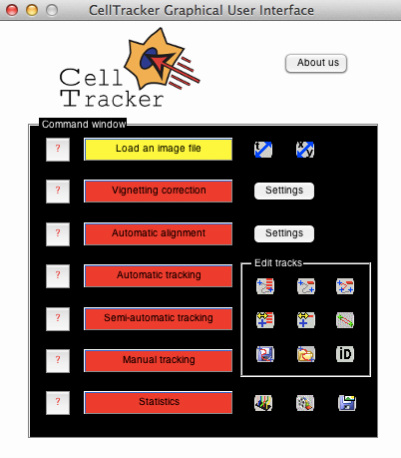
Upon typing “CellTrackerGUI” in the Matlab command window, the following window appears:
At the initialization step, the functionality buttons (e.g. vignetting correction, automatic tracking, etc.) appear in red, and progressively change their colour while the tracking process moves forward.
Explanation of the colours:
· RED: this operation cannot be performed yet. For example, vignetting correction is not possible if there is no image loaded.
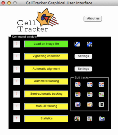
· YELLOW: the operation may be performed. In the case of the tracking functionality buttons, even after the specific operation is performed, the button stays yellow, meaning that it is possible to add new tracks.
· GREEN: the operation has already been performed, no post-action required/possible (except for the button "Load an image file").
LOAD AN IMAGE FILE
Click “Load an image file” button to open images. This will open a window for browsing folders. In order to load an image file (CellTracker accepts TIFF, AVI, and BioFormats files), select a file and click “Open”. The image file must contain at least two frames in order to perform tracking. After an image is loaded, the “Load an image file” button becomes green and all the other dialog buttons will turn to yellow, indicating that the user may now proceed with the next steps. In order to open a new image, simply click again this button.
CROP IMAGES (in X-Y or time)

Crop the image in x-y. The user must draw a rectangle around the region to be kept. Only the selected region will remain.

Cropping image sequences over time (i.e. remove some frames). A window will be prompted to the user, where the desired first and last frame can be chosen.
IMAGE PRE-PROCESSING
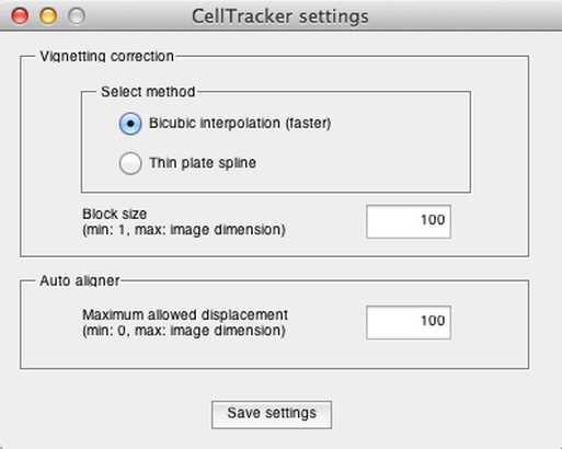
Two different pre-processing steps may be performed: "Vignetting correction" and "Automatic alignment". Parameters of these steps can be adjusted by clicking the “Settings” button.
Vignetting correction
The basic method of correcting uneven signal intensity distributions in the images is to reconstruct a reference image from the background and use this reference to flat-field correct the original images. We implemented two methods:
Bicubic interpolation: an image downscale-upscale method, which assumes there are no objects larger than a few pixels, it is the faster method and generally works well.
Thin plate spline: it is rather slow but more accurate in approximating the background. If modification needed, choose the block size to be at least twice as big than the usual object size on the image. Note: Matlab “Curve Fitting Toolbox” is required to perform this method.
The "Block size" parameter (expressed in pixels) should be greater than the diameter of a typical cell.
Automatic alignment
The images acquired in time-lapse experiments are often not perfectly aligned in x-y due to paraxial shifts of the microscope stage. The image alignment method uses cross-correlation. This removes image shaking, given that the objects are stationary or the cell movement direction is uniformly distributed. It is possible to set the expected maximum pixel distance between two consecutive images in the "Settings" menu.
AUTOMATIC TRACKING
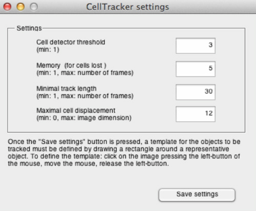
CellTracker is capable of detecting cells automatically based on template matching. Tracking starts in the current frame and ends in the last frame of the image sequence. Once the "Automatic tracking" button is pressed, a window will be prompted to the user, allowing modification of several parameters.
Cell detector threshold: if this is set too high, the cells will not be detected. If it is too low, debris will potentially be considered as cells. Briefly: the AVERAGE intensity across the image is computed and the cells to be tracked are defined as the objects having higher intensity than "THRESHOLD x AVERAGE".
Memory (for cells lost): maximal number of frames still considered when a tracked cell becomes temporarily undetected (e.g. it goes out of focus or out of the field of view).
Minimal track length: minimum number of frames a tracked cell is included in the analysis. Tracks shorter (i.e. having less number of frames) than the set value will be automatically discarded.
Maximal cell displacement: maximal expected displacement (distance measured in pixels) between consecutive frames. The value of this parameter is fundamental in obtaining good results. To estimate its proper value, it is recommended to open two consecutive images of the image set with an external image-processing program, like ImageJ (http://rsbweb.nih.gov/ij/), and measure the displacement for several cells. We suggest that the user sets the "maximal cell displacement" to the maximum of these values or slightly bigger. Too large values can result mismatches in track assignments, while too small values result errors in tracking fast objects.
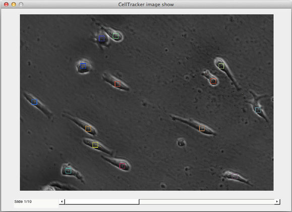
After all the parameters are set, click “Save settings” to select a representative template. Draw a rectangle around a representative cell/object. Once the template is defined, the tracking starts immediately. The resulting tracks are displayed as coloured squares outlining each tracked cell.
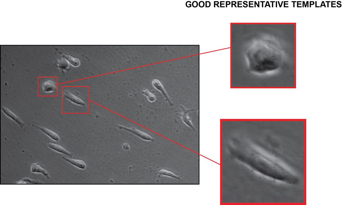
Guideline for template selection:
The choice of template is fundamental to obtain good results. There is no “golden rule” to define the most representative template; however, we try to give a cookbook here based on our experiences. Several attempts may be needed to find a template providing good results. Generally, an isolated cell (i.e. not surrounded by other cells), with similar morphology to most of the cells, would be a good candidate. Often, cells with different morphologies can be present on the image. Accordingly, we suggest that before the real tracking scenario the user tries different templates. In case of unsuccessful trial, all the tracks can be easily deleted and start again with a better template. It is worth noting that more templates can be used for the same image series. According to our experience, the tracking of mixed cell populations can be started by concentrating first on one of the cell morphologies then by clicking the "Automatic tracking" again, adding other morphologies. Multiple detections of a single cell or tracks that are wrongly computed can be simply deleted by using the track editing buttons: "Merge two tracks" and "Remove track(s)" (for more details see Section "EDIT TRACKS MENU" below).
SEMI-AUTOMATED TRACKING
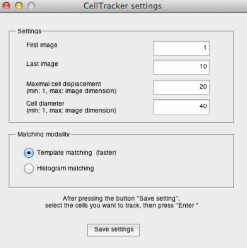
This button allows the user to track cells in a semi-automated fashion. In this case, the cells to be tracked are selected by the user. The first and the last frame tracked may be defined in a pop-up menu. Two input parameters are required: the "Maximal cell displacement" (see description in the "Automatic tracking" section) and the approximate "Cell diameter" (measured in pixels).
Then, it is possible to select multiple cells, by simply clicking on them. Selected cells will be marked with white crosses. Cells too close to the image borders will not be tracked. The tracking step is started upon pressing “Enter”.Individual tracks are shown as coloured squares overlaying tracked cells. If the "Template matching" modality (faster) is selected, a cell will be recognized by using a rectangular template defined around the selected cell. Otherwise, if the "Histogram matching" modality is selected, a cell on the consecutive frame is recognized by finding the best local histogram match.
MANUAL TRACKING
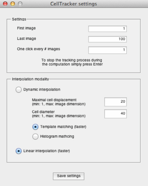
This option allows the user to manually track a cell in the designated time interval (from the first to the last selected image) using given temporal step size (i.e. the number of images skipped between mouse clicks). The skipped time points will be automatically computed accordingly to the interpolation technique selected. If the "Linear interpolation" modality is selected, the missing coordinates will be linearly interpolated between the user-defined coordinates. Otherwise, if the "Dynamic interpolation" modality is selected, the missing coordinates will be computed using a so-called dynamic programming technique, which finds the globally optimal path between the user defined coordinates by quickly calculating the cost of all possible pathways. The input parameters required in this case are already explained in the above "Automatic tracking" and "Semi-automatic tracking" sections. Once the settings were defined, to create a new track, press the "Manual tracking" button, move the mouse over the centroid of the cell you want to track, and click. The slider and the displayed image will be updated upon this action. If the manual tracking should be terminated before the last set frame, simply press "Enter".
EDIT TRACKS MENU
The buttons on this menu allow the user to remove, merge, save, and load tracks.

Remove all the tracks. All computed tracks will be deleted.

Remove track(s). Removes one or more selected tracks. Select the
tracks to be removed with a left-click, and press “Enter”.

Remove track(s) from the current timepoint. Removes the selected track (or multiple tracks) starting from the given timepoint, keeping the earlier parts of the selected tracks.

Move track with a fixed shift from the current timepoint. Allows the user to redefine the coordinates of a track from a given timepoint, applying a fixed shift.

Move a single point of a track. Allows the user to redefine the coordinates of a track at a given timepoint by simply clicking on the new coordinate.

Merge two tracks.The tracks to be merged must be
present simultaneously at least in one frame. If they are not, use the
"Manual tracking" button to connect the two tracks. The first
mouse-click will select the first track fragment, while the second mouse-click will
select the second track fragment. When both of the fragments are present in a
given time point, their geometric centre will be the new track at that time
point.

Saves tracking coordinates as a .mat file.The saved file contains 4 columns: coordinate
x, coordinate y, timepoint, track ID. By selecting the above icon, the location
and the filename of this temporary file can be controlled and saved.

Loads previously saved tracks. The file loaded must contain 4
columns: coordinate x, coordinate y, timepoint, track ID. Loading a data file
removes all current tracks.

Change track ID. Every track is uniquely identified by a positive integer number, called
Identification Number (ID). This button allows to visualize the ID of a track, and to change the track ID.
Identification Number (ID). This button allows to visualize the ID of a track, and to change the track ID.
STATISTICS
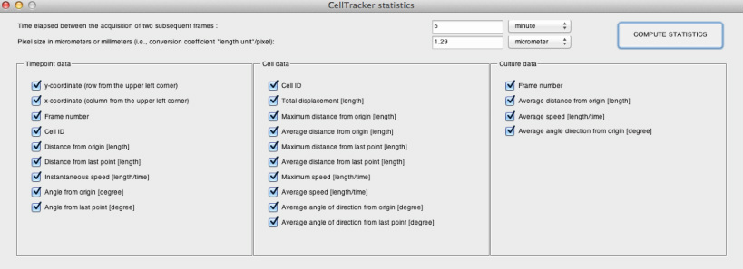
It is possible to calculate and export several statistical measures about:
Data of different timepoints: contains variables describing individual tracks (i.e. tracked cells) in every timepoint (i.e. frame).
Cell data: combined data of each track throughout the computed timepoints (one row per track).
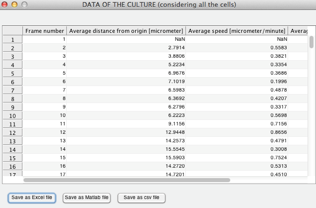
Culture data: data averaged over the tracked cell population (i.e. all the cells combined) for every timepoint.
The desired statistics can be selected by ticking specific boxes.
Before calculating the statistics, the user can optionally define the "time elapsed between the acquisition of subsequent frames" (units: second, minute, hour, days) and the "pixel size in micrometers or millimeters". If these parameters are defined, the software returns statistics computed accordingly.
The results can be exported as XLS, MAT and CSV files, enabling further processing with other software tools. Note for Macintosh users: file export in XLS format is not supported; instead the results will be saved as CSV. In this case, the file header will be lost. As a solution, we suggest saving the statistics computed also as MAT file, and copy the column headers from the "ColumnNames" variable.
What follows is a brief description of some of the measures computed. It is worth noting that in our reference the coordinate of the upper-left-corner (ULC) pixel of the image is (1, 1).
What follows is a brief description of some of the measures computed. It is worth noting that in our reference the coordinate of the upper-left-corner (ULC) pixel of the image is (1, 1).
Timepoint data: x-coordinate and y-coordinate.
Timepoint data: distance from origin. For each cell the origin is the position of the cell at timepoint 1 (i.e. first frame from which the cell is tracked).
Timepoint data: distance from last point.
Timepoint data: instantaneous speed: distance from the last point divided by the time elapsed between the acquisition of two subsequent frames.
Timepoint data: angle from origin: angles in degree (between 0° and 359°) of the red arrows shown in the figure on the right.
Timepoint data: angle from last point: angles in degree of the red arrow
Cell data: total displacement: length of the red path.
Cell data: maximum distance from origin.
Cell data: average distance from origin: average of the lengths of the red arrows that represent the distance of the cell from origin for each timepoint.
Cell data: maximum distance from last point.
Cell data: average distance from last point: average of the lengths of the red arrows.
Timepoint data: average angle of direction from origin: average of the angles of the red arrows.
Timepoint data: average angle of direction from last point: average of the angles of the red arrows.
Finally, several buttons for visualization of the tracks computed are available:

3D tracks plot. Displays all the tracks over time in a x-y-z plot, where the z axis represents the time.

Create a video. Creates an AVI video, where the tracked are displayed with coloured squares.

Save
the current stack of images. Saves the current image stack as a TIFF
file. The saving can be performed at any stage of the tracking process.

